Many moons ago I did a first post exploring the non-obvious logic of the most secretive of Tableau table calculation configuration options: At the Level. A few weeks ago I was inspired by a question over email to dive back in, this post explores At the Level for the five rank functions: RANK(), RANK_DENSE(), RANK_MODIFIED(), RANK_UNIQUE(), and RANK_PERCENTILE(). The rank functions add a level of indirection to the already complicated behavior of At the Level and I don’t have any particular use cases, so…

The particular challenge with ordinal functions like INDEX(), FIRST(), and the rank functions is that we absolutely have to understand how addressing and partitioning works in Tableau, and then we tack onto that an understanding of how the calculations work, and finally we can add on how At the Level works. For the first part, I suggest you read the Part 1 post on At the Level, it goes into some detail on addressing and partitioning. To understand the rank functions here’s the Tableau manual for table calculations (scroll down to the Rank functions section). Finally, read on for how At the Level works for rank functions.

Order of Operations for At the Level for Rank Functions

There are 6 steps that I’ve identified for how Tableau computes rank functions that use At the Level. I’m going to quickly list these, then there are several examples below that walk through each step. Note that the order of steps is being performed within each “true” partition created by the partitioning dimension(s).

1. We start out with what I’m calling for now temp partitions based on the dimension used for At the Level and the addressing dimensions above it in the partitioning & addressing dialog. (If you don’t know what the partitioning & addressing dialog is, then stop here and study the links in Want to Learn Table Calculations).One way to think of the temp partitions is that they are like a set of queues, one queue per each unique combination of values of the At the Level & higher addressing dimension, like a set of check-out lines at a grocery store.
2. The distinct combinations of values of the dimension(s) in the view create the addresses aka rows in the partition. In this case the dimension(s) that are below At the Level are effectively creating the addresses in each temp partition.
3. The first address in each temp partition as defined by the dimension sort of the view is the 1st position, 2nd address is the 2nd position, and so on, so these are creating ordinal positions. To use the check-out line metaphor the ordinal position identifies the 1st person in each queue/temp partition, 2nd person in each queue, and so on.
4. The ordinal positions are then used to create ordinal partitions, in other words the bucket/group/slice of all the addresses that are going to be ranked together. So all of the addresses in the 1st ordinal position create one ordinal partition, all of the addresses in the 2nd position create the 2nd ordinal partition, and so on. In the check-out line this would be grouping together into the 1st ordinal partition everyone who is 1st in each queue, then everyone who is 2nd in each queue goes into the 2nd ordinal partition, and so on.
5. The addresses in each ordinal partition are sorted according to the measure used for the RANK function, restarting for each ordinal partition. This is where the RANK calcs head in a different direction from other table calcs because they do their own sort of the partition. In the check-out line if we were doing something like RANK(SUM([Number of Items])) then everyone who is 1st in each queue would get sorted based on the SUM([Number of Items]), then everyone who is 2nd in each queue would get sorted, and so on.
6. Finally the ranking is applied to each address, restarting for every new ordinal partition.

Example 1: Simple Data

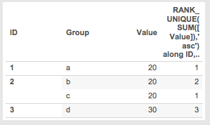
This data set is set up with 4 records, with two dimensions, ID & Group. The view has ID and Group in it and RANK_UNIQUE(SUM([Value]),’asc’) is set to have a Compute Using on ID & Group, At the Level ID. Since all dimensions in the view are part of the addressing there is only one “true” partition.

Image may be NSFW.
Clik here to view.

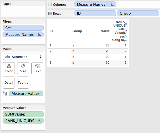
1. There are three “temp partitions” based on ID 1, 2, 3.
2. There are 4 addresses aka rows in the partition, with two for ID 2 due to groups a and b.
3. Here’s how the ordinal positions end up:
   • ID 1 Group a is in temp partition 1, position 1
   • ID 2 Group b is in temp partition 2, position 1
   • ID 2 Group c is in temp partition 2, position 2 (it’s the 2nd address in temp partition 2)
   • ID 3 Group d is in temp partition 3, position 1
     Image may be NSFW.
     Clik here to view.
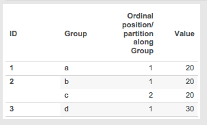
4. Now the ordinal partitions are created based on the positions:
   • ID 1 Group a is in ordinal partition 1
   • ID 2 Group b is in ordinal partition 1
   • ID 3 Group d is in ordinal partition 1
   • ID 2 Group c is in ordinal partition 2
     Image may be NSFW.
     Clik here to view.
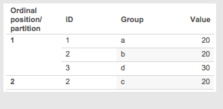
5. The ordinal partitions are sorted by the measure, then alphanumerically for the dimensions in case of ties:
   • Ordinal partition 1
     • Value 20 ID 1 Group a
     • Value 20 ID 2 Group b
     • Value 30 ID 3 Group d
   • Ordinal partition 2
     • Value 20 ID 2 Group a
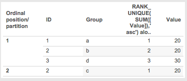
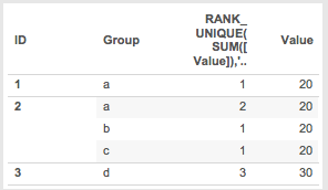
6. The RANK_UNIQUE is applied:
   • Ordinal partition 1
     • Rank 1 Value 20 ID 1 Group a
     • Rank 2 Value 20 ID 2 Group b
     • Rank 3 Value 30 ID 3 Group d
   • Ordinal partition 2
     • Rank 1 Value 20 ID 2 Group cImage may be NSFW.
       Clik here to view.

Then when we go back to the view with just ID and Group as dimensions the ranks may seem nonsensical in their ordering but in fact there’s a very specific logic that led to those results:
Image may be NSFW.
Clik here to view.

Example 2: Adding a Record to Simple Data

In this case I’ve added an address for ID 2 Group a with a Value of 20. This means that there are now 3 positions because there are 3 separate groups in ID 2, so ultimately there will be three separate ordinal partitions:

Image may be NSFW.
Clik here to view.

Here’s how the ordinal partitions work out for step 6:

• Ordinal partition 1
  • Rank 1 Value 20 ID 1 Group a
  • Rank 2 Value 20 ID 2 Group a
  • Rank 3 Value 30 ID 3 Group d
• Ordinal partition 2
  • Rank 1 Value 20 ID 2 Group b
• Ordinal partition 3
  • Rank 1 Value 20 ID 2 Group c

Here’s what it looks like in a view just sorted by ID and Group, the ranks only look odd because of the use of At the Level:
Image may be NSFW.
Clik here to view.

Example 3: Rank and At the Level for Discrete Dimensions

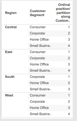
This example uses Superstore with Region & Customer Segment (called Segment from here on out) as the dimensions where the calc will be RANK_UNIQUE(MIN([Region]),’asc’) with an Advanced Compute Using on Region & Segment, At the Level Region. I’ve filtered out South/Consumer to make the data set sparse. I find using dimension values to be helpful in explaining what is going on because then we can just deal with the alpha sort on the dimension, in this case Region.

Here’s the result of the calc:

Image may be NSFW.
Clik here to view.

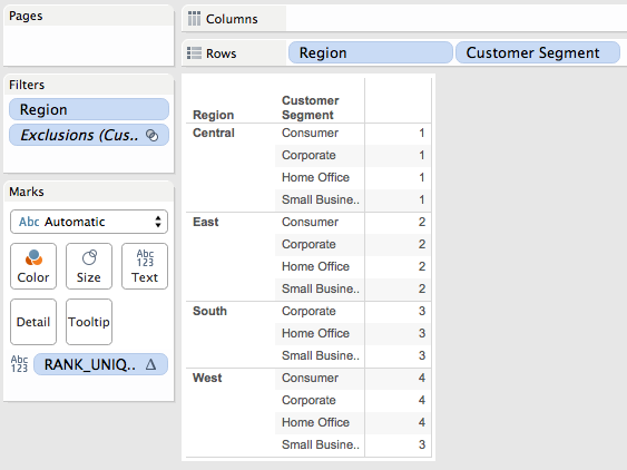
The reason why West/Small Business gets a 3 is due to the same process I’ve outlined above, I’ll walk through it:

1. There are 4 temp partitions on Region: Central, East, South, and West.
2. There are 15 addresses (only three Customer Segments in South, all others have 4 Segments).
3. The temp partition addresses with the ordinal position number are as follows. Note how the ordinal positions for South have different Customer Segment assignments than the other Regions:
   Image may be NSFW.
   Clik here to view.
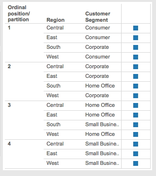
4. Now here are ordinal partitions:
   Image may be NSFW.
   Clik here to view.
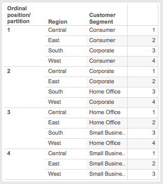
5. The ordinal partitions are sorted by the measure, in this case MIN([Region)]). That doesn’t change anything in this case from step 4 above.
6. The ranks are applied in each ordinal partition(you can see this in the R/S Rank worksheet):
   Image may be NSFW.
   Clik here to view.

Again, this just to help demonstrate how the process works, I’m not sure when I’d ever use this in practice.

Dates, Rank, and At the Level

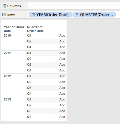
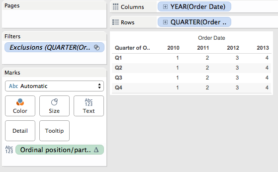
Now for some explorations of dates, rank functions, and at the level as a continuation of the discrete dimension exploration. This is where things can be a little funkier than they’ve gotten already because we need to be careful of whether we’re using date parts (as in just the year, quarter, day of month, etc.) or date values aka datetrunc’s like 2015-01-01 12:00am (year), 2015-09-01 12:00am (month), 2015-09-17 12:00am (day), 2015-09-17 8:00am (hour), etc. For these examples I’m using Superstore again, the dimensions are the dateparts Quarter of Order Date and Year of Order Date with 2010 Q3 filtered out of the data.

Image may be NSFW.
Clik here to view.

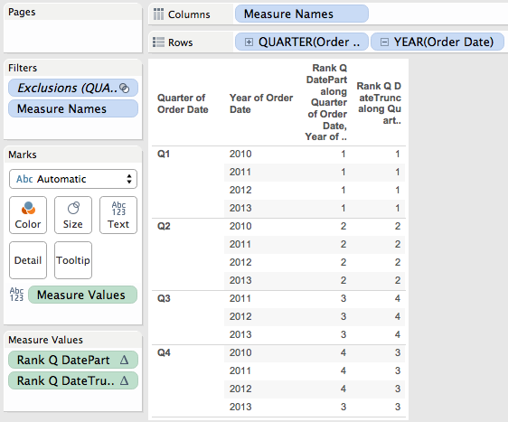
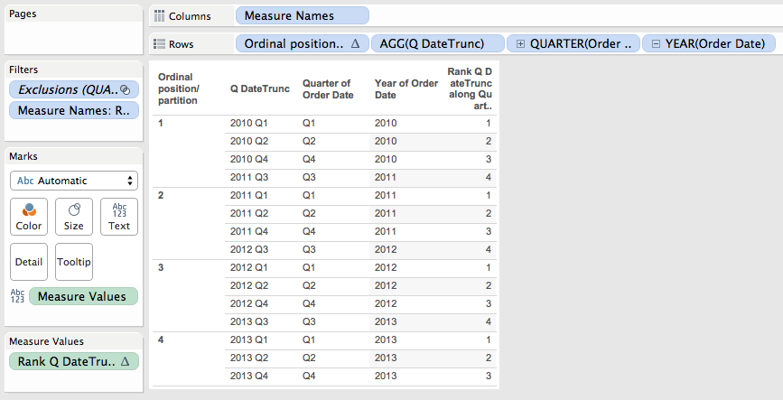
Here’s a pic of the different results of two rank calcs, one uses the formula RANK_UNIQUE(DATEPART(‘quarter’,MIN([Order Date])), ‘asc’) and the other is RANK_UNIQUE(DATETRUNC(‘quarter’,MIN([Order Date])), ‘asc’), both have an Advanced… Compute Using on Quarter of Order Date, Year of Order Date At the Level Quarter of Order Date:

Image may be NSFW.
Clik here to view.

Weird, eh?

Example 4: Rank and At the Level for Date Parts

I’ll walk through the datepart version first, so in this case the quarter is really Q1, Q2, Q3, Q4.

1. There are 4 temp partitions for Q1, Q2, Q3, Q4.
2. There are 15 addresses since 2010 Q3 has been filtered out.
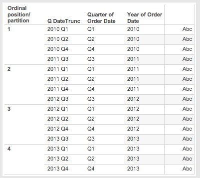
3. The temp partition addresses with the ordinal position number are as follows (you can also see this in the Q/Y Ordinal Position worksheet:)
   Image may be NSFW.
   Clik here to view.
4. Now here are ordinal partitions (you can see this in the Q/Y Ordinal Partition worksheet):
   Image may be NSFW.
   Clik here to view.
5. The ordinal partitions are sorted by the measure, in this case DATEPART(‘quarter’,MIN([Order Date])). That doesn’t change anything in this case from step 4 above.
6. The ranks are applied in each ordinal partition(you can see this in the Q/Y Rank for DatePart worksheet):
   Image may be NSFW.
   Clik here to view.

So that missing 2010/Q3 value causes the 3rd position in each ordinal partition to be offset by a year in the data, which then ultimately changes the ranks.

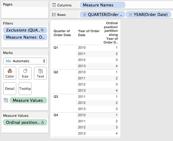
Example 5: Rank and At the Level for Date Value

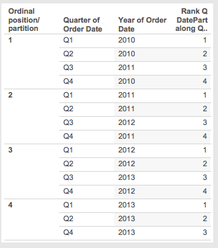
Now for the datevalue, where the rank calc is RANK_UNIQUE(DATETRUNC(‘quarter’,MIN([Order Date])), ‘asc’) so the DATETRUNC() is returning 2010-01-01, 2010-04-01, etc. The first 4 steps in the calculation are *exactly* the same as previous because the dimensions in the view are the same. So when we get to step 4, here are the ordinal partitions:

4. Now here are ordinal partitions (you can see this in the Q/Y Ordinal Partition worksheet):
   Image may be NSFW.
   Clik here to view.
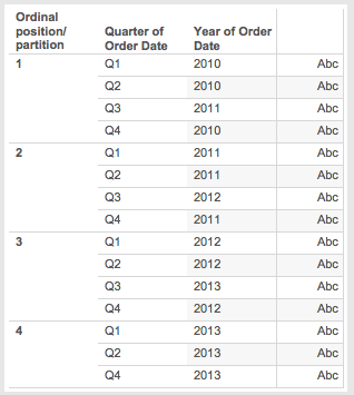
5. The ordinal partitions are sorted by the measure, in this case DATETRUNC(‘quarter’,MIN([Order Date])). You can see this in Q/Y Sort for DateTrunc, the sort is different from when we used the datepart because instead sorting on just the quarter we’re now sorting on the year *and* quarter.
   Image may be NSFW.
   Clik here to view.
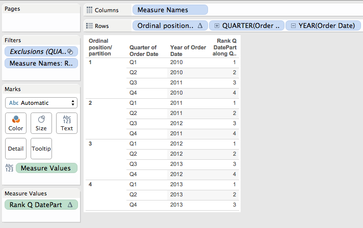
6. Finally the RANK_UNIQUE is applied, here’s the sorted partitions and rank. You can see this in the Q/Y Rank for DateTrunc:
   Image may be NSFW.
   Clik here to view.

Warning About Domain Completion

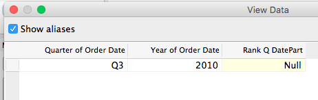
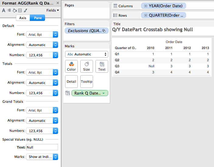
In the Q/Y Rank for DatePart worksheet the Rank for DatePart for 2010 Q4 is 4:

Image may be NSFW.
Clik here to view.

However if I change the layout to a crosstab with Quarter on Rows and Year on Columns then 2010 Q4 gets a rank of 3, you can see that in the Q/Y DatePart Crosstab Problem worksheet:
Image may be NSFW.
Clik here to view.
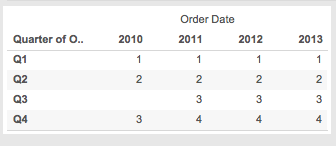
The reason why is domain completion. In the original Q/Y Rank for DatePart worksheet there are 15 marks. In the Q/Y DatePart Crosstab Problem worksheet above. there are 16 marks because the pill layout and presence of the Rank table calculation are triggering domain completion and Tableau is padding in a mark for 2010 Q3. One way to identify that is to right-click on that cell and choose View Data… In the View Data window the yellow cell for Rank Q DatePart indicates that it has been padded in by Tableau.
Image may be NSFW.
Clik here to view.
Here’s how Tableau ends up with results in this case:

1. There are 4 temp partitions for Q1, Q2, Q3, Q4.
2. There are 16 addresses since even though 2010 Q3 has been filtered out it has been padded back in by domain completion.
3. The temp partition addresses with the ordinal position number are as follows – note that 2010 Q3 gets the 3rd position even though it doesn’t exist in the underlying data, it’s only from the padding that it exists:
   Image may be NSFW.
   Clik here to view.
4.  The ordinal partitioning ends up with a partition for each year.
5. Next, Tableau sorts the partition, in this case by DATEPART(‘quarter’,MIN([Order Date])). However the MIN([Order Date]) for 2010 Q3 doesn’t exist in the data so that returns Null (even in the padded data), changing the sort.
6. Finally the RANK_UNIQUE is computed, here’s the sorted partitions and rank. Since the RANK calcs ignore Nulls, RANK_UNIQUE returns Null for 2010 Q3 (I’m showing this by turning on Special Value formatting):
   Image may be NSFW.
   Clik here to view.

So that’s an example of how rank calcs with At the Level can get changed by Tableau’s densification behaviors. The easiest solution is the “remove densification” trick originally discovered by Joe Mako where we move all the dimensions on Rows/Columns/Pages to the Level of Detail Shelf and use corresponding aggregate measures to get the right layout, in this case I created a couple of date fields for the Year & Quarter with some custom number formatting and wrapped them in the ATTR() aggregation.

Image may be NSFW.
Clik here to view.

Conclusion

Rank functions add a whole new level of indirection to At the Level. If your data set is domain complete then this behavior wouldn’t necessarily affect you, however if your data set is sparse then the results are unlikely to be what you are looking for. If you have any particular use cases for rank functions and At the Level I’d love to know them, please respond in the comments below!

Here’s the At the Level for Rank functions workbook on Tableau Public.